
Using Grafana
Overview
Grafana is an open-source BI tool managed by Grafana Labs. We utilize Grafana as our default demo BI tool. However, directions for other BI tools, such as Microsoft’s PowerBI, can be found in our North Bound services section.
- Using Grafana, users can visualize time series data using pre-defined dashboards.
- Details on how to use Grafana to visualize data in the network are available in the Using Grafana document.
- Example configurations and dashboards can be found at import grafana dashboard document.
Prerequisites & Links
- Grafana Documentation
- Grafana Install - We support Grafana 9.5.16 or higher.
- The REST service enabled on the EdgeLake node (the Query Node) that services the Grafana Request.
- Use the following command on the EdgeLake CLI to enable the REST service:
<run rest server where
    external_ip=!external_ip and external_port=!anylog_rest_port and
    internal_ip=!ip and internal_port=!anylog_rest_port and
    bind=!rest_bind and threads=!rest_threads and timeout=!rest_timeout
>
Note:
[ip]and[port]are the IP and Port that would be available to REST calls.[max time]is an optional value that determines the max execution time in seconds for a call before being aborted.- A 0 value means a call would never be aborted and the default time is 20 seconds.
Setting Up Grafana
- Login to Grafana - The default HTTP port that Grafana listens to is 3000 - On a local machine go to
http://localhost:3000.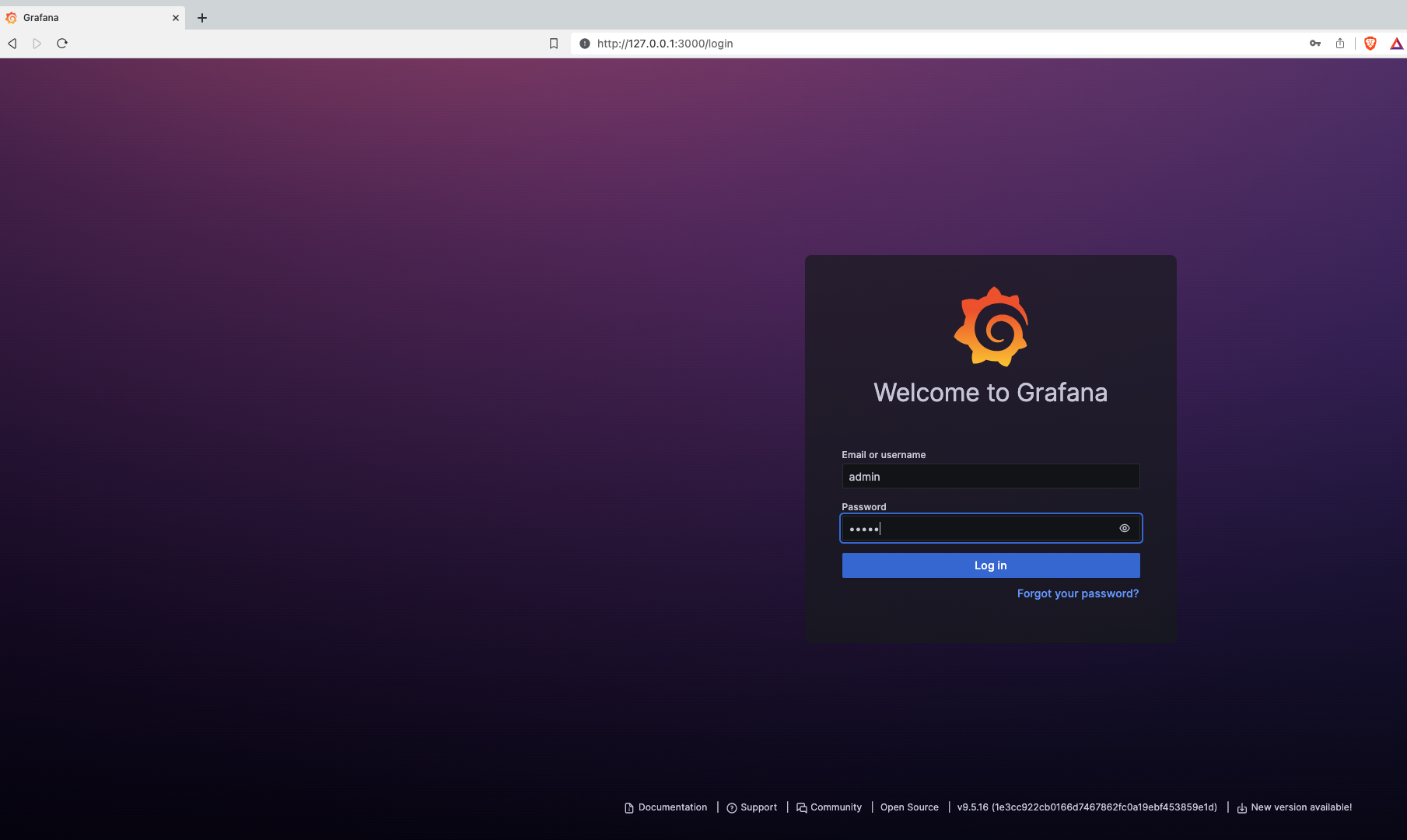
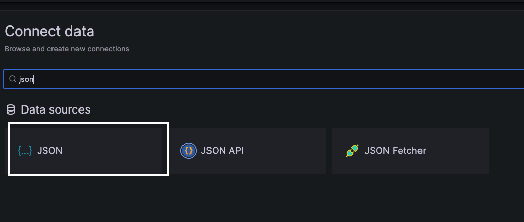
- In Data Sources section, create a new JSON data source
- Select a JSON data source
- On the name tab provide a unique name to the connection.
- On the URL Tab add the REST address offered by the EdgeLake node (i.e. http://10.0.0.25:32149)
- On the Custom HTTP Headers, name the default database. If no header is set, then all accessible databases to the node will be available to query
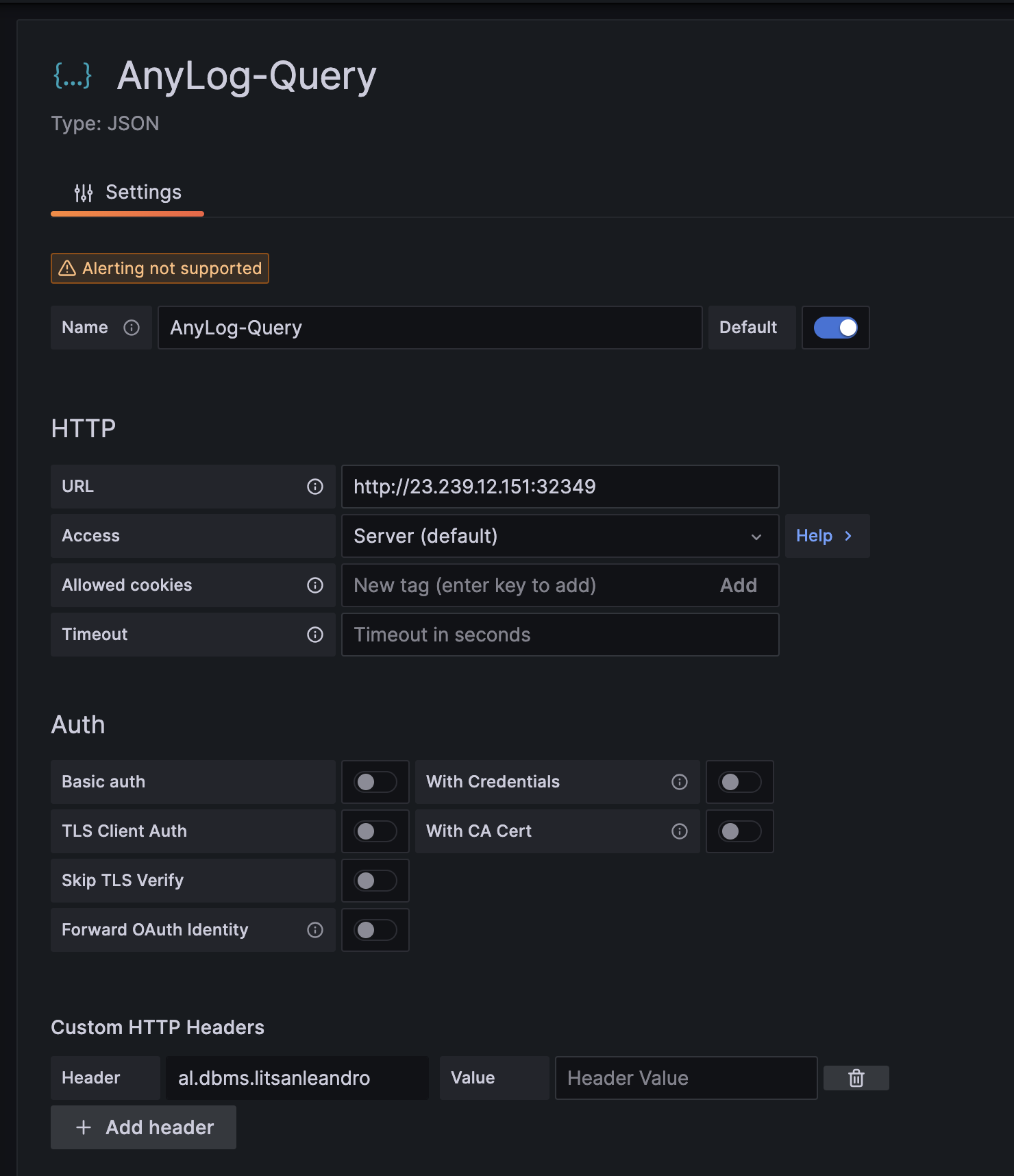
- Select the Save and Test option that should return a green banner message: ***Data source is working***.

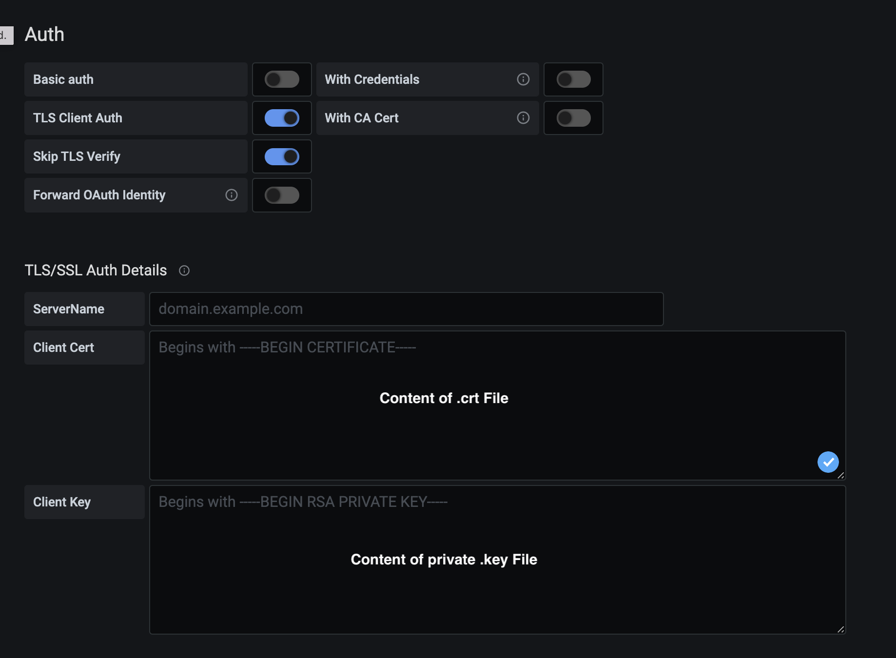
Enabling Authentication
Enabling authentication is explained at Authenticating HTTP requests.
- For Basic Authentications, the Grafana configuration should have basic auth enabled.
- Basic Authentications validates username and password, details are at basic authentication.
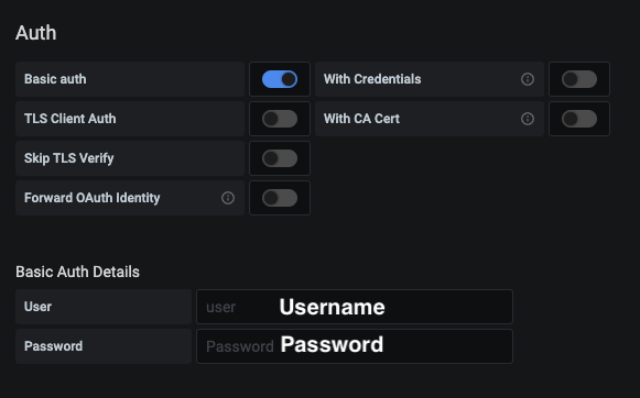
- Using certificates is detailed in SSL Certificates.
- On Grafana, set TLS Client Auth and Skip TLS Verify enabled.
Notes: Failure to connect may be the result of one of the following
- EdgeLake instance is not running or not configured to support REST calls.
- Wrong IP and Port.
- Firewalls are not properly configured and the needed IP and Port not available.
- EdgeLake is configured with authentication detection that is not being satisfied.
- If Grafana is properly connected, the database and tables of the EdgeLake network can be selected on the Grafana GUI. If Gragfana fails to connect, the dashboard (Edit Panel/Metric Selection) presents “Error: No table connected” in the pull-down menu.
Using Grafana to visualize EdgeLake data
Grafana allows to present data in 2 modes Time Series collects and visualize data values as a function of time, and Table format where data is presented in rows and columns.
EdgeLake queries are represented in the Grafana JSON API, and details of the configuration are available here. Queries are represented in the JSON API using one of the following methids:
- As a SQL query.
- As a push-down Increment function.
- As a push-down period function.
The push-down functions are very efficient as processing are fone on the edge and only summaries are returned on the network.
The query information is represented using JSON in the Payload section. The Grafana info including the Payload is transferred to the EdgeLake query node, where it is transforms to a query that is executed on the nodes in the network.
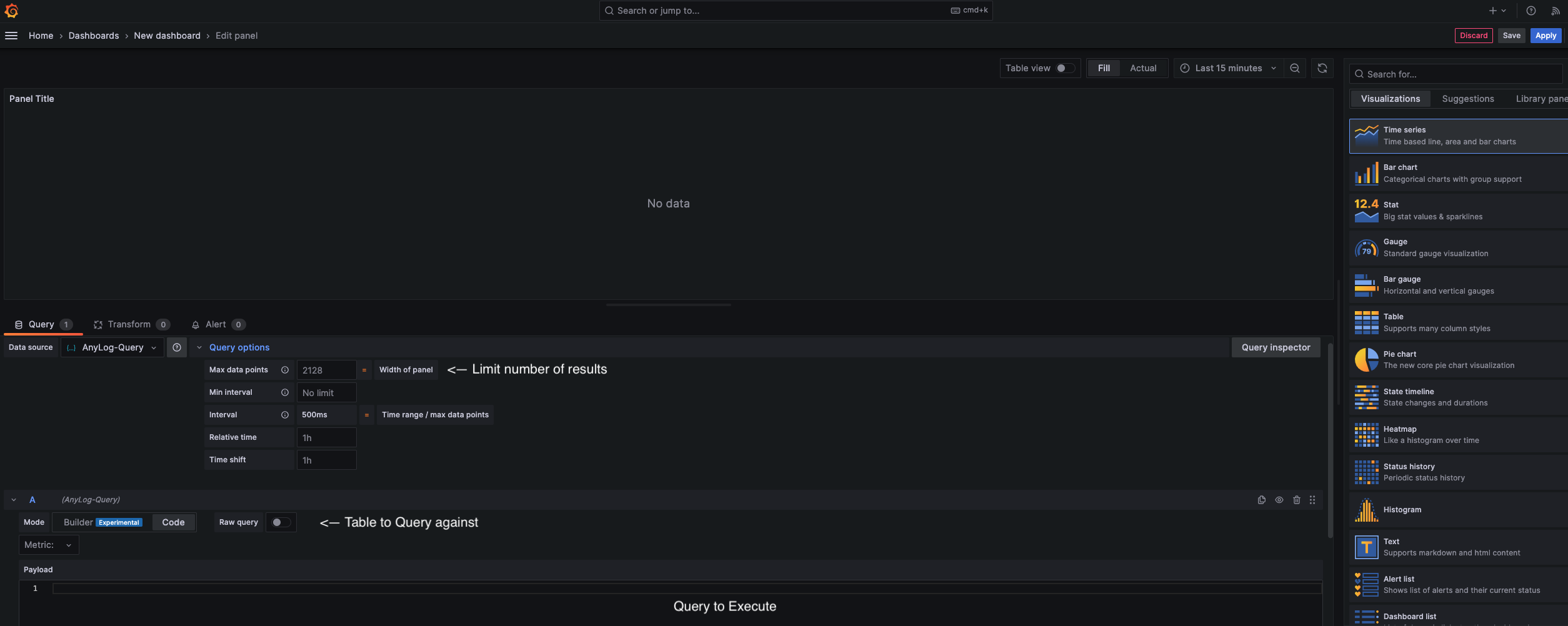
To represent a query, follow the following steps for each Panel:
- Select the JSON data Source.
- Select the logical database and table from the pull down menu in the Metric section.
- Represent the EdgeLake query in the Payload section.
The chart below summarized the attribute names for the JSON payload:
| dbms | The name of the logical database to use. Overrides the dbms name in the configuration page. |
| table | The name of the table to use. Overrides the table name in the sql statement. |
| type | The type of the query. The default value is 'sql' and other valid types are: 'increments', 'period' and 'info'. |
| sql | A sql statement to use. |
| details | An EdgeLake native command which is not a SQL statement. |
| where | A "WHERE" condition added to the SQL statement. Can add filter or other conditions to the executed SQL. |
| functions | A list of SQL functions to use which override the default functions. |
| time_column | The name of the time column in the Time Series table. |
| value_column | The name of the value column in the Time Series table. |
| time_range | When using a Table view, determines if the query needs to consider the time range. The default value is 'true'. |
| servers | Replacing the network determined Operators (nodes hosting data) with a list of user determined Operators to use. |
| instructions | Additional EdgeLake query instructions. |
| trace_level | By setting debug level to 1, the executed query and the number of rows returned are printed on the Query Node CLI. |
| timezone | Overwrite the default timezone. Note that the same timezone needs to be set on the Grafana dashboard. See details in the **Timezone considerations** section below. |
| interval | Overwrite the intervals calculated by the query process. See details in the increment function detailed below. |
| grafana:format_as | Determines the format of the returned values. |
| grafana:data_points | The value fixed presents the returned values using the Grafana Intervals (as detailed in the Query options section. See details in the section **Fixed data points** below. |
Timezone considerations
When a query is issued from the Grafana Dashboard, the timezone is selected by the user (in the dropdown timerange menu). The grafana timezone options might not be consistent with the timezones options supported by EdgeLake and if needed, users can specify the timezone in the JSON Payload section.
For example, Grafana can issue the value “browser” as a timezone (to indicate that the timezone of the browser is selected). However, the query node can be deployed in a different timezone which may lead to inconsistencies.
By adding a timezone attribute and a value in the JSON payload, users can associate between the Grafana timezone abbreviation and EdgeLake timezone abbreviation. Note that EdgeLake returns the values in the target timezone, and the Grafana timezone needs to represent the same timezone as EdgeLake.
The list of timezone abbreviations used by EdgeLake is available here.
The following are additional abbreviation for EdgeLake:
- utc - utc timezone
- pt - America/Los_Angeles
- mt - America/Denver
- ct - America/Chicago
- et - America/New_York
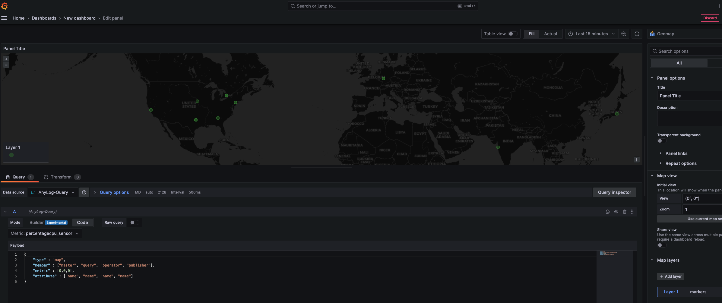
Metadata based Visualization - A Network Map
In the Visualizations section, select Geomap
In the Metric section, select a table name to “query” against
Update Payload with the following information
{
    "type" : "map",
    "member" : ["master", "query", "operator", "publisher"],
    "metric" : [0,0,0],
    "attribute" : ["name", "name", "name", "name"]
}
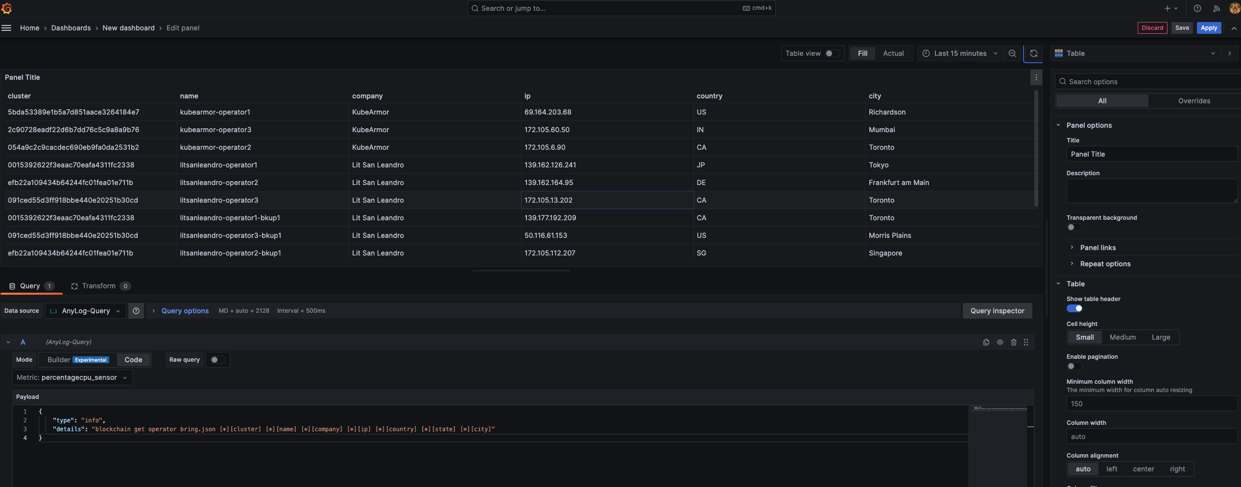
Metadata based Visualization - Visualizing Blockchain Data (Metadata)
In the Visualizations section, select Table
In the Metric section, select a random table - the JSON instruction will override the selction.
Update Payload with the following information
{
    "type": "info",
    "details": "blockchain get operator bring.json [*][cluster] [*][name] [*][company] [*][ip] [*][country] [*][state] [*][city]"
}
SQL Query
The following SQL query returns the last values ingested by the database. Note that without the limit, the entire table’s data is returned, and even if a time range is added, it may include a huge number of rows.
The increment and period pushdown functions detailed below consider all relevant data while also allowing control over the volume of data returned.
Example SQL query:
SELECT
  timestamp, a_current, b_current, c_current
FROM
  bf
WHERE
  id = 1
ORDER BY
  timestamp DESC
LIMIT 1
Example JSON Payload:
{
  "sql": "select timestamp, a_current, b_current, c_current from bf where id = 1 order by timestamp desc limit 1;"
}
Example Gauge with latest values: 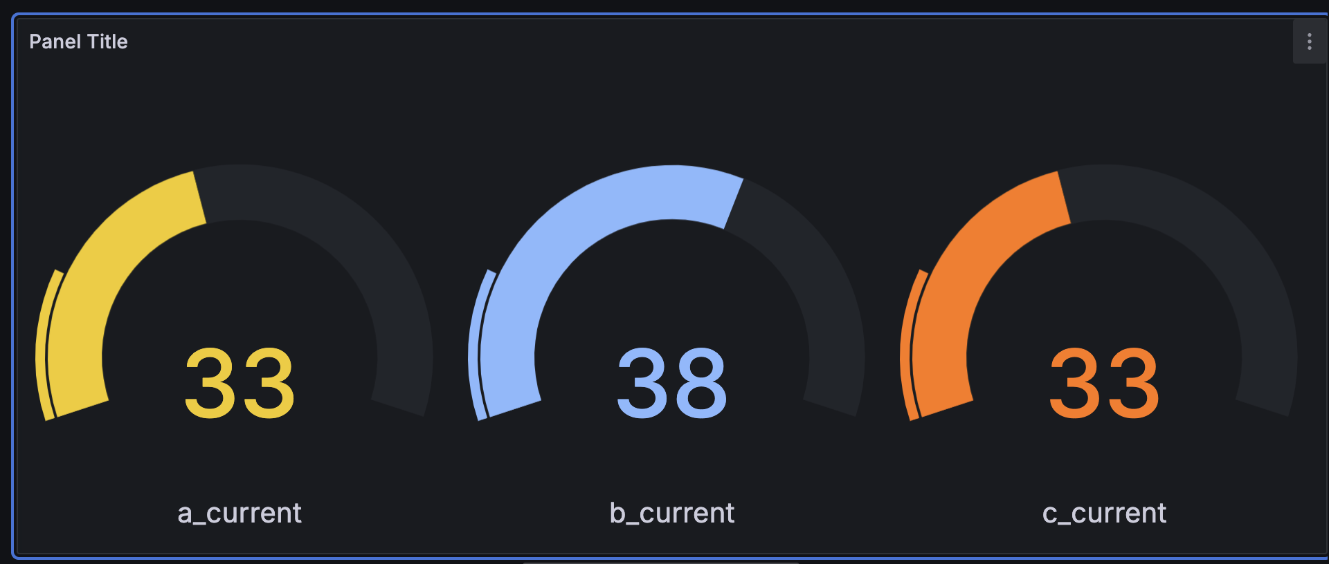
The Increment Query
Increments query (The default query) is used to retrieve statistics on the time series data in the selected time range. Depending on the number of data point requested, the time range is divided to intervals and the min, max and average are collected for each interval and graphically presented.
- In the Visualizations section, select Time series
- In the Metric section, select a table name to “query” against
- Update Payload with the following information
# Input in Grafana { "type": "increments", "time_column": "timestamp", "value_column": "value", "grafana": { "format_as": "timeseries" } } - Under Query Options, update Max data points (limit value), and see comment below (Considering the Grafana limit).
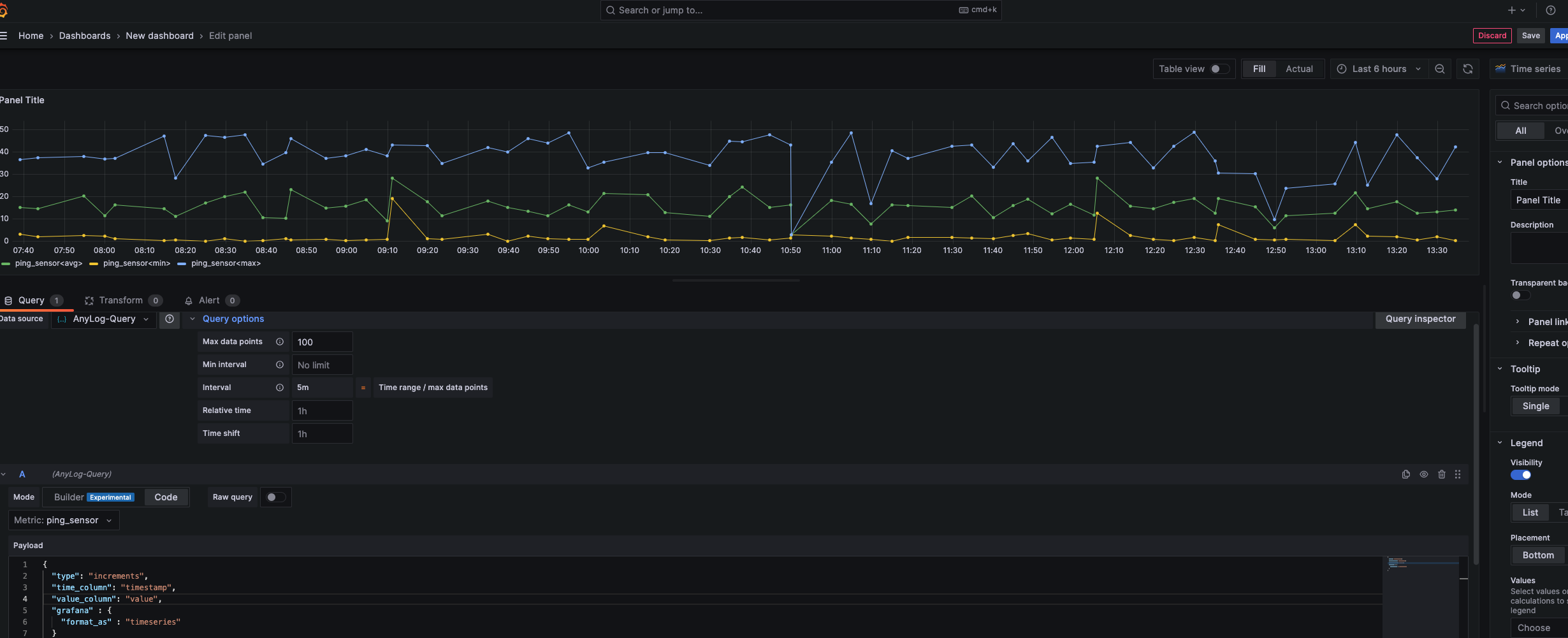
When the query type is set to increments, the query being executed on the EdgeLake side is as follows:
SELECT
  increments(second, 1, timestamp), max(timestamp) as timestamp, avg(value) as avg_val, min(valu e) as min_val,
  max(value) as max_val
FROM
  percentagecpu_sensor
WHERE
  timestamp >= '2024-02-19T19:42: 02.133Z' and timestamp <= '2024-02-19T19:57:02.133Z'
LIMIT 2128;
Understanding and Tuning Increments queries
The increment function allows to push processing to the edge nodes and return summaries. This is a very powerful way to query data for the following reasons:
- Rows are processed concurrently by multiple edge nodes.
- Only summaries are transferred over the network as well as keeping the Grafana memory usage contained.
An increment query is executed on each participating node as follows:
- A time range is divided to intervals.
- All the rows in the time range are visited and evaluated.
- For each interval, the selected query functions are calculated (min, max, average, count, sum).
- A single entry is returned for each time interval.
- The query node unifies the replies from all the participating nodes to a unified result.
The number of time points returned
The number of points returned to an increment function determines on the time intervals that are considered.
With Grafana, 3 options are available:
- Not specifying the time intervals - in this case, EdgeLake will determine an optimized time interval.
- Specifying a time interval (in the JSON Payload using the attribute key interval with the interval value, for example: “interval” : “3 minutes”, or in the query statement, for example: increments(minute,1,timestamp)).
- Using the time intervals provided by Grafana (specify the value: dashboard for the key interval).
To see the optimized value, add "trace_level" : 1 to the JSON Payload. The Query node displays the increment details.
Here is an output example where a point is returned for every 1 hour interval:
DEBUG
Process: [0:Success] Rows: [248] Details: [increments(hour, 1, insert_timestamp)]
Stmt: [run client () sql cos timezone = local SELECT increments(insert_timestamp), max(insert_timestamp) as timestamp , avg(chemicalscale4ai_pv) as avg_val from cos_wp_analog where insert_timestamp >= '2024-07-26T20:08:44.761Z' and insert_timestamp <= '2024-07-27T02:08:44.761Z' limit 1260;]
To query with a different time interval, specify the interval in the JSON Payload.
The following example overwrites the optimized setting with a user defined interval.
In the example below, each data point represents 10 minutes interval and provides to Grafana the average min and max values for each 10 minutes (note also that the Payload includes the trace option enabled):
JSON
{
  "type": "increments",
  "time_column": "insert_timestamp",
  "value_column": "chemicalscale4ai_pv",
  "functions": ["avg", "min", "max"],
  "grafana": {
    "format_as": "timeseries"
  },
  "interval" : "10 minutes",
  "trace_level" : 1

}
Fixed data points
The fixed data points option considers the number of data points specified in the Grafana Query options.
With this option, the returned data (by an increment function) aligns with the Grafana derived interval (see the Time Range/max data points value in the Query options of the Grafana dashboard).
For every interval, a data point is returned, and if no data point exists in the interval, a null value is returned.
In the example below, data_points are set to fixed to indicate a returned value (or null) for each time interval and the interval attribute maintains the value dashboard to indicate that the intervals are to leverage the values from the Grafana dashboard.
{
  "type": "increments",
  "time_column": "insert_timestamp",
  "value_column": "hw_influent",
  "functions": ["avg"],
  "grafana": {
    "format_as": "timeseries",
    "data_points" : "fixed"
  },
  "1timezone": "pt",
  "interval" : "dashboard",
  "trace_level" : 1
}
Considering the Grafana limit
When Grafana issues a query it will include a limit. Users need to make sure that the limit is not lower than the number of points returned.
Note that the trace option provides the info on the number of points returned to Grafana. Using the defaults (and not specifying intervals that overwrite the defaults) with a limit to set to 1000 or higher, will always return all the needed values.
The Period Query
Period query is a query to retrieve data values at the end of the provided time range (or, if not available, before and nearest to the end of the time range).
The derived time is the latest time with values within the time range. From the derived time, the query will determine a time interval that ends at the derived time and provides the avg, min and max values.
To execute a period query, include the key: ‘type’ and the value: ‘period’ in the Additional JSON Data section.
- In the Visualizations section, select Gauge
- In the Metric section, select a table name to “query” against
- Update Payload with the following information
# Input in Grafana { "type": "period", "time_column": "timestamp", "value_column": "value", "grafana" : { "format_as" : "timeseries" } } - Under Query Options, update Max data points (ie limit) otherwise the outcome would look like a single line as opposed to clearly showing min / max / avg value(s).
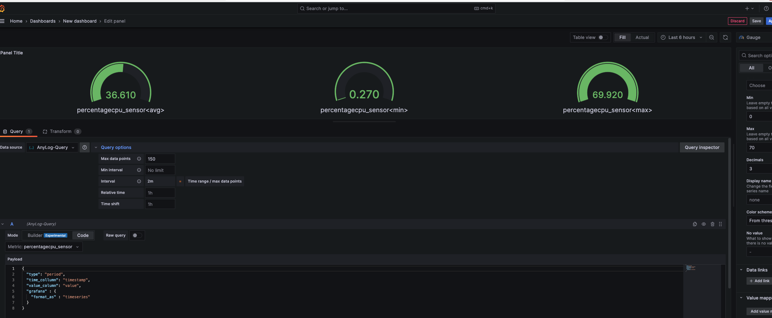
When the query type is set to period, the query being executed on the EdgeLake side is as follows:
SELECT
    max(timestamp) as timestamp, avg(value) as avg_val, min(value) as min_val, max(value) as max_val
FROM
    ping_sensor
More information on increments and period types of queries are available in queries and info requests.
Other Grafana Examples
- Extending query to use where conditions
{
  "type": "increments",
  "time_column": "timestamp",
  "value_column": "value",
  "where": "device_name='ADVA FSP3000R7'",
  "grafana" : {
    "format_as" : "timeseries"
  }
}- Example without where conditions
{
  "type": "period",
  "time_column": "timestamp",
  "value_column": "value",
  "time_range": false,
  "functions": ["min", "max", "avg", "count"],
  "grafana" : {
    "format_as" : "timeseries"
  }
}
Monitoring and Trace Options
Tracing Grafana Queries
Users can trace queries that are generated from the Grafana panels as follows:
- By setting debug level to 1, the executed query and the number of rows returned are printed on the CLI of the node that services Grafana.
This setting enables trace on the specific queries where trace_level is set.
Example:
{
  "sql": "SELECT insert_timestamp, servicepump1running_di FROM cos_wp ORDER BY insert_timestamp DESC limit 1",
  "time_range": false,
  "timezone": "local",
  "trace_level" : 1
}- Trace of all the queries from the Grafana instance can be enabled using the trace level command on the CLI of the Query Node:
trace level = 1 grafanaSetting trace level to 0 disables the trace.
Queries time statistics
Users can view statistics on the queries execution time using the following command:
get queries time
Users can reset the statistics using the following command:
reset query timer
Identifying slow queries
Slow queries can be redirected to the query log with the following command:
set query log profile [n] seconds
Whereas [n] is a threshold in seconds. Queries with execution time higher than the threshold will be logged to the query log.
Use the following command to log all queries to the query log:
set query log
Use the following command to retrieve the query log:
get query log
Use the following command to reset the query log:
reset query log
Info on a query execution
Users can drill to specific queries to find how the query was executed using the following command:
query status
Additional information is available int the Profiling and Monitoring Queries section.